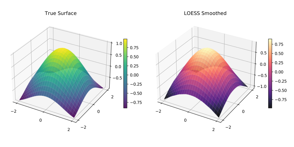
Standard LOESS operates on a single predictor \(x\). Setting dimensions > 1 extends the neighbourhood search and local polynomial fit into an \(n\)-dimensional predictor space, enabling surface smoothing over spatial grids, time–altitude combinations, and similar multi-predictor datasets.
Dimensions
Use Case
Input Shape
1
Time series, 1D signal (default)
x: 1-D array
2
Spatial surface, 2-predictor model
x: n × 2 matrix
3+
High-dimensional regression
x: n × d matrix
Computational cost
Neighbourhood search scales with \(d\) dimensions. For dimensions ≥ 3 keep fraction small and consider increasing delta to activate interpolation.
Two predictors (e.g., latitude/longitude, time/altitude). Pass an \(n \times 2\) matrix as x.
# n × 2 predictor matrixcoords<-cbind(lat,lon)model<-Loess(dimensions=2L,fraction=0.3)result<-model$fit(coords,z)
importnumpyasnpimportfastloessasfl# x is an (n, 2) array flattened to 1D (Python binding requires flat input)x2d=np.column_stack([lat,lon]).ravel()model=fl.Loess(dimensions=2,fraction=0.3)result=model.fit(x2d,z)
// x is an (n × 2) row-major matrixfastloess::LoessOptionsd2_opts;d2_opts.dimensions=2;d2_opts.fraction=0.3;fastloess::Loessmodel(d2_opts);autoresult=model.fit(x2d,z).value();