Skip to content

Polynomial Degree

Degree of the local polynomial fitted at each point.

Overview

At each target point, LOESS fits a polynomial to the neighbouring data using weighted least squares. The degree parameter controls the order of that polynomial.

Degree Comparison

Degree Local Fit Captures Risk
0 Constant Level only Over-smooth, biased at edges
1 Linear Trend (default) Rarely overfits
2 Quadratic Curvature Overfits with small fraction
3 Cubic Inflections Requires larger fraction
4 Quartic Fine structure High variance, rarely needed

Degree 0 — Local Constant

\[\hat{y}(x_0) = \arg\min_a \sum_i w_i(x_0)\,(y_i - a)^2\]

The fit at each point is simply a weighted mean. Produces very smooth results but ignores local slope, introducing bias wherever the true function changes.

Use when: Maximum smoothness is more important than accuracy; computationally cheapest option.

model <- Loess(degree = 0L, fraction = 0.5)
result <- model$fit(x, y)
model = fl.Loess(degree="constant", fraction=0.5)
result = model.fit(x, y)
let model = Loess::new()
    .degree("constant")
    .fraction(0.5)
    .build()?;
let result = model.fit(&x, &y)?;
model = Loess(; degree="constant", fraction=0.5)
result = fit(model, x, y)
const model = new Loess({ degree: 0, fraction: 0.5 });
const result = model.fit(x, y);
const model = new Loess({ degree: "constant", fraction: 0.5 });
const result = model.fit(x, y);
fastloess::LoessOptions deg0_opts;
deg0_opts.degree = "constant";
deg0_opts.fraction = 0.5;
fastloess::Loess model(deg0_opts);
auto result = model.fit(x, y).value();

Degree 1 — Local Linear (Default)

\[\hat{y}(x_0) = \arg\min_{a,b} \sum_i w_i(x_0)\,(y_i - a - b x_i)^2\]

Fits a weighted line through the neighbourhood. Removes first-order bias and handles boundary regions correctly. The right choice for the vast majority of applications.

Use when: Default; monotone or gently curved data; boundary accuracy matters.

model <- Loess(degree = 1L, fraction = 0.5)
result <- model$fit(x, y)
model = fl.Loess(degree="linear", fraction=0.5)
result = model.fit(x, y)
let model = Loess::new()
    .degree("linear")
    .fraction(0.5)
    .build()?;
let result = model.fit(&x, &y)?;
model = Loess(; degree="linear", fraction=0.5)
result = fit(model, x, y)
const model = new Loess({ degree: 1, fraction: 0.5 });
const result = model.fit(x, y);
const model = new Loess({ degree: "linear", fraction: 0.5 });
const result = model.fit(x, y);
fastloess::LoessOptions deg1_opts;
deg1_opts.degree = "linear";
deg1_opts.fraction = 0.5;
fastloess::Loess model(deg1_opts);
auto result = model.fit(x, y).value();

Degree 2 — Local Quadratic

\[\hat{y}(x_0) = \arg\min_{a,b,c} \sum_i w_i(x_0)\,(y_i - a - b x_i - c x_i^2)^2\]

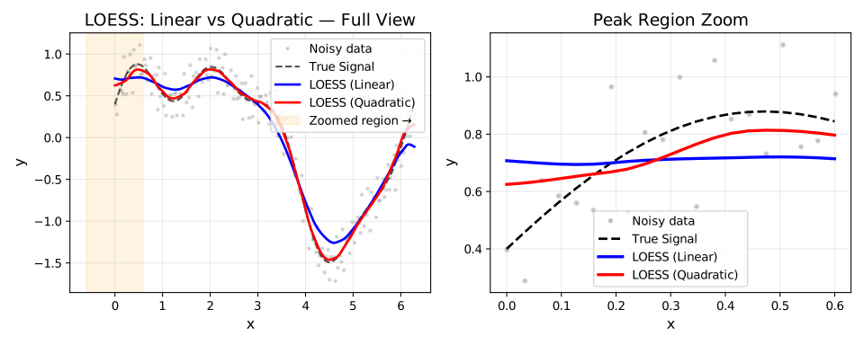
Fits a weighted parabola through the neighbourhood. Removes second-order bias and captures local curvature more faithfully, but requires more data per neighbourhood — pair with a larger fraction (≥ 0.4) to avoid overfitting.

Use when: Data with pronounced peaks, valleys, or curvature; fraction ≥ 0.4.

model <- Loess(degree = 2L, fraction = 0.5)
result <- model$fit(x, y)
model = fl.Loess(degree="quadratic", fraction=0.5)
result = model.fit(x, y)
let model = Loess::new()
    .degree("quadratic")
    .fraction(0.5)
    .build()?;
let result = model.fit(&x, &y)?;
model = Loess(; degree="quadratic", fraction=0.5)
result = fit(model, x, y)
const model = new Loess({ degree: 2, fraction: 0.5 });
const result = model.fit(x, y);
const model = new Loess({ degree: "quadratic", fraction: 0.5 });
const result = model.fit(x, y);
fastloess::LoessOptions deg2_opts;
deg2_opts.degree = "quadratic";
deg2_opts.fraction = 0.5;
fastloess::Loess model(deg2_opts);
auto result = model.fit(x, y).value();

Degree 3 — Local Cubic

\[\hat{y}(x_0) = \arg\min_{a,b,c,d} \sum_i w_i(x_0)\,(y_i - a - b x_i - c x_i^2 - d x_i^3)^2\]

Fits a weighted cubic polynomial. Captures inflection points and S-shaped local behaviour. Requires a substantially larger neighbourhood than degree 2 — use fraction ≥ 0.5 and verify visually for overfitting.

Use when: Data has clear S-shaped curves or multiple inflection points; fraction ≥ 0.5.

model <- Loess(degree = 3L, fraction = 0.6)
result <- model$fit(x, y)
model = fl.Loess(degree="cubic", fraction=0.6)
result = model.fit(x, y)
let model = Loess::new()
    .degree("cubic")
    .fraction(0.6)
    .build()?;
let result = model.fit(&x, &y)?;
model = Loess(; degree="cubic", fraction=0.6)
result = fit(model, x, y)
const model = new Loess({ degree: 3, fraction: 0.6 });
const result = model.fit(x, y);
const model = new Loess({ degree: "cubic", fraction: 0.6 });
const result = model.fit(x, y);
fastloess::LoessOptions deg3_opts;
deg3_opts.degree = "cubic";
deg3_opts.fraction = 0.6;
fastloess::Loess model(deg3_opts);
auto result = model.fit(x, y).value();

Degree 4 — Local Quartic

\[\hat{y}(x_0) = \arg\min_{a,...,e} \sum_i w_i(x_0)\,(y_i - a - b x_i - \cdots - e x_i^4)^2\]

Fits a weighted quartic polynomial. Rarely needed in practice; only useful for capturing highly oscillatory local structure. Very prone to overfitting — require fraction ≥ 0.6 and cross-validate.

Use when: Fine oscillatory structure is physically meaningful and the dataset is large; always cross-validate.

model <- Loess(degree = 4L, fraction = 0.7)
result <- model$fit(x, y)
model = fl.Loess(degree="quartic", fraction=0.7)
result = model.fit(x, y)
let model = Loess::new()
    .degree("quartic")
    .fraction(0.7)
    .build()?;
let result = model.fit(&x, &y)?;
model = Loess(; degree="quartic", fraction=0.7)
result = fit(model, x, y)
const model = new Loess({ degree: 4, fraction: 0.7 });
const result = model.fit(x, y);
const model = new Loess({ degree: "quartic", fraction: 0.7 });
const result = model.fit(x, y);
fastloess::LoessOptions deg4_opts;
deg4_opts.degree = "quartic";
deg4_opts.fraction = 0.7;
fastloess::Loess model(deg4_opts);
auto result = model.fit(x, y).value();

Choosing the Right Degree

Situation Recommended Degree
Monotone trend, general purpose 1 (default)
Maximum smoothness, speed 0
Clear peaks / valleys / inflections 2 (with fraction ≥ 0.4)
S-shaped curves, multiple inflections 3 (with fraction ≥ 0.5)
Fine oscillatory structure (rare) 4 (with fraction ≥ 0.6, cross-validate)
Boundary accuracy is critical 1 or 2 (not 0)
Very small dataset (n < 50) 1

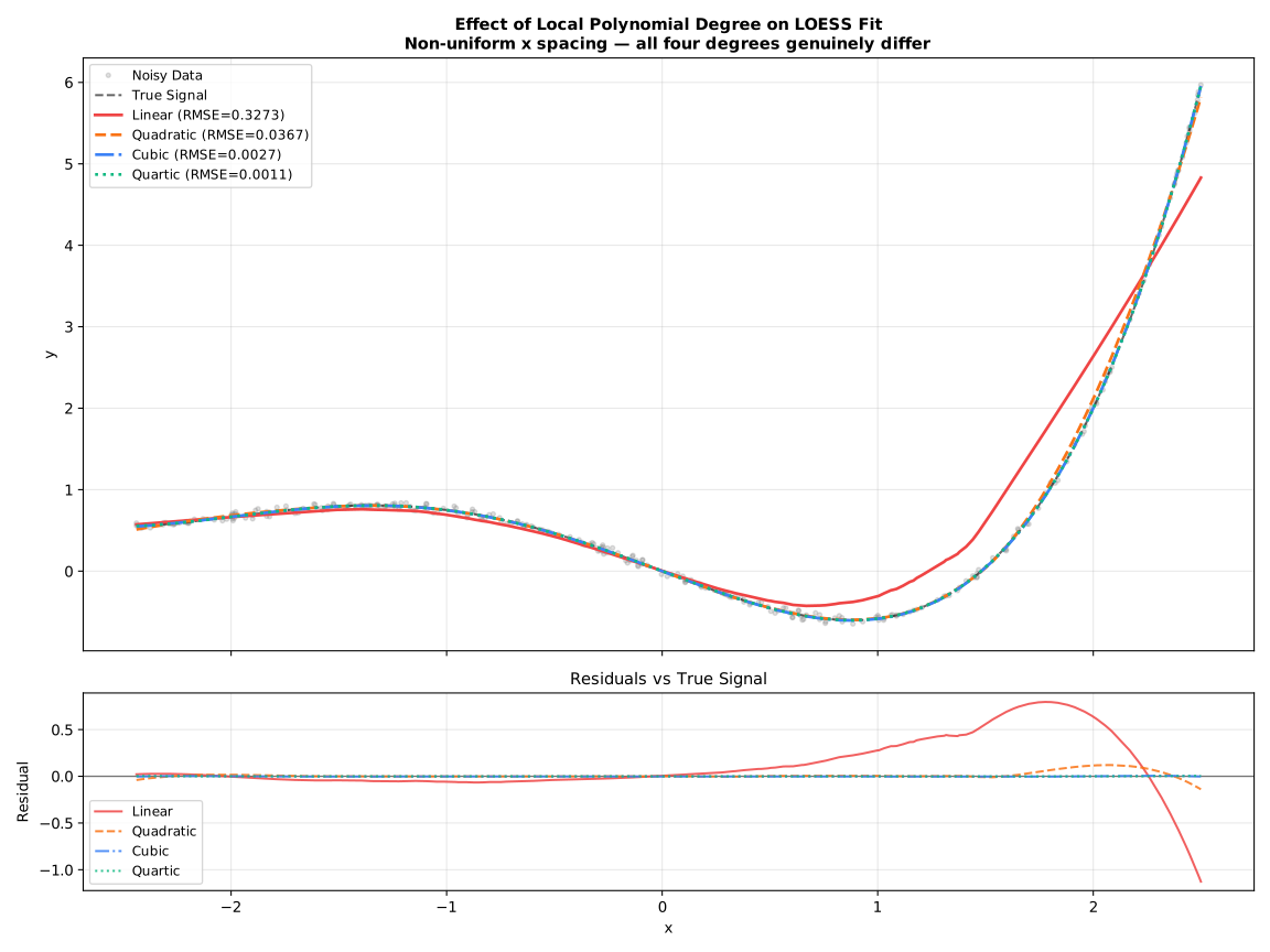
Higher Degree Effects

Higher Degree Comparison


Surface Mode

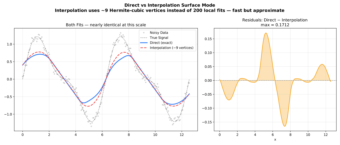
The surface_mode parameter controls whether LOESS evaluates the local polynomial at every query point or at a sparser grid of vertices with Hermite cubic interpolation in between.

Mode Behaviour Speed Accuracy
"interpolation" (default) Evaluate at anchor vertices, blend via Hermite cubic Faster Slight approximation
"direct" Evaluate at every query point Exact Full precision

Surface Mode Comparison

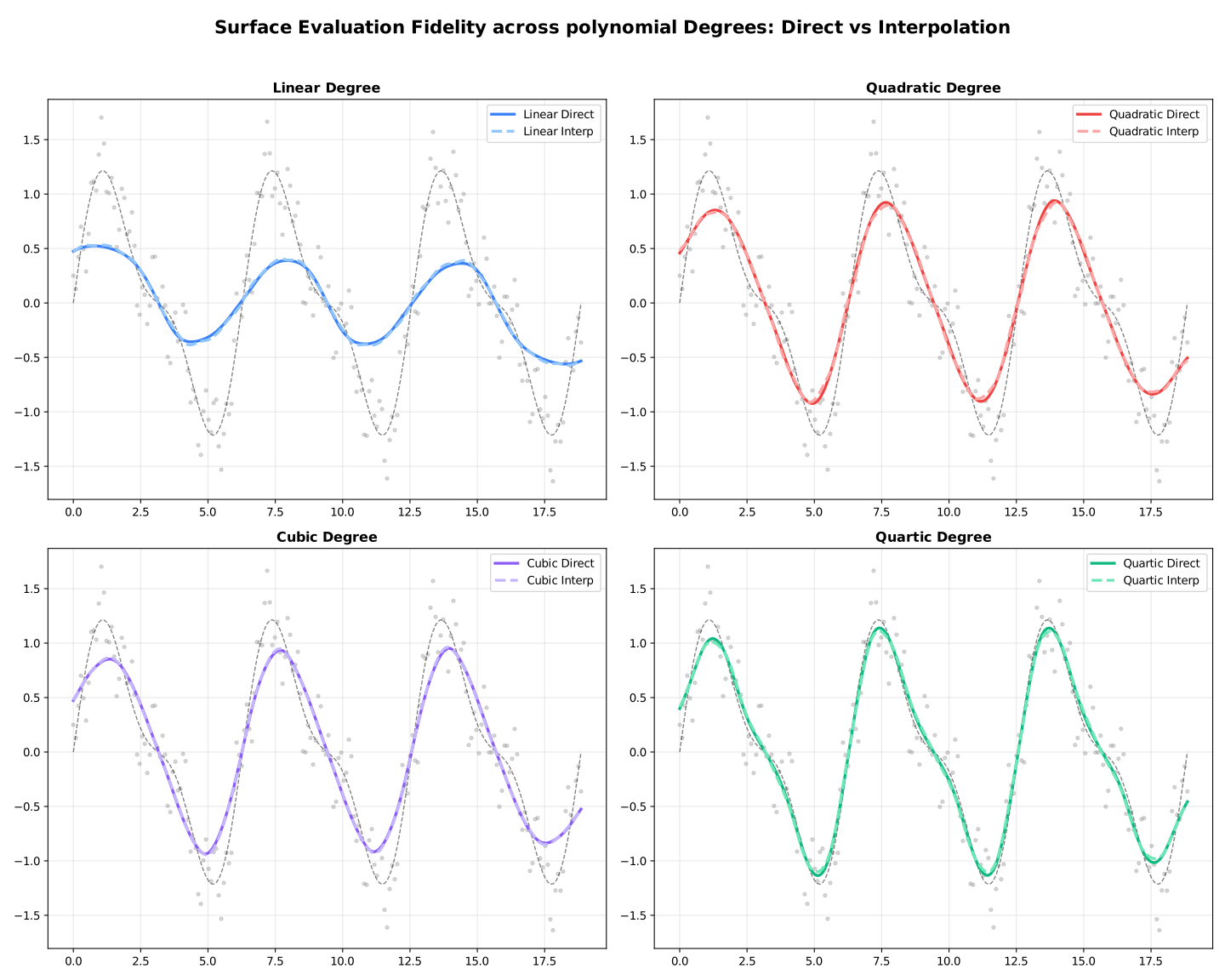
Degree × Interpolation