Concepts
Understanding how LOESS works and when to use it.
What is LOESS?
LOESS (Locally Estimated Scatterplot Smoothing) is a nonparametric regression method that fits smooth curves through scatter plots without assuming a global functional form.
Unlike parametric methods (linear regression, polynomial fitting), LOESS adapts locally to the data structure, making it ideal for:
- Exploratory data analysis — Discover patterns without assumptions
- Trend estimation — Extract signals from noisy time series
- Baseline correction — Remove systematic effects in spectroscopy
- Genomic smoothing — Smooth methylation, ChIP-seq, or expression data
How It Works
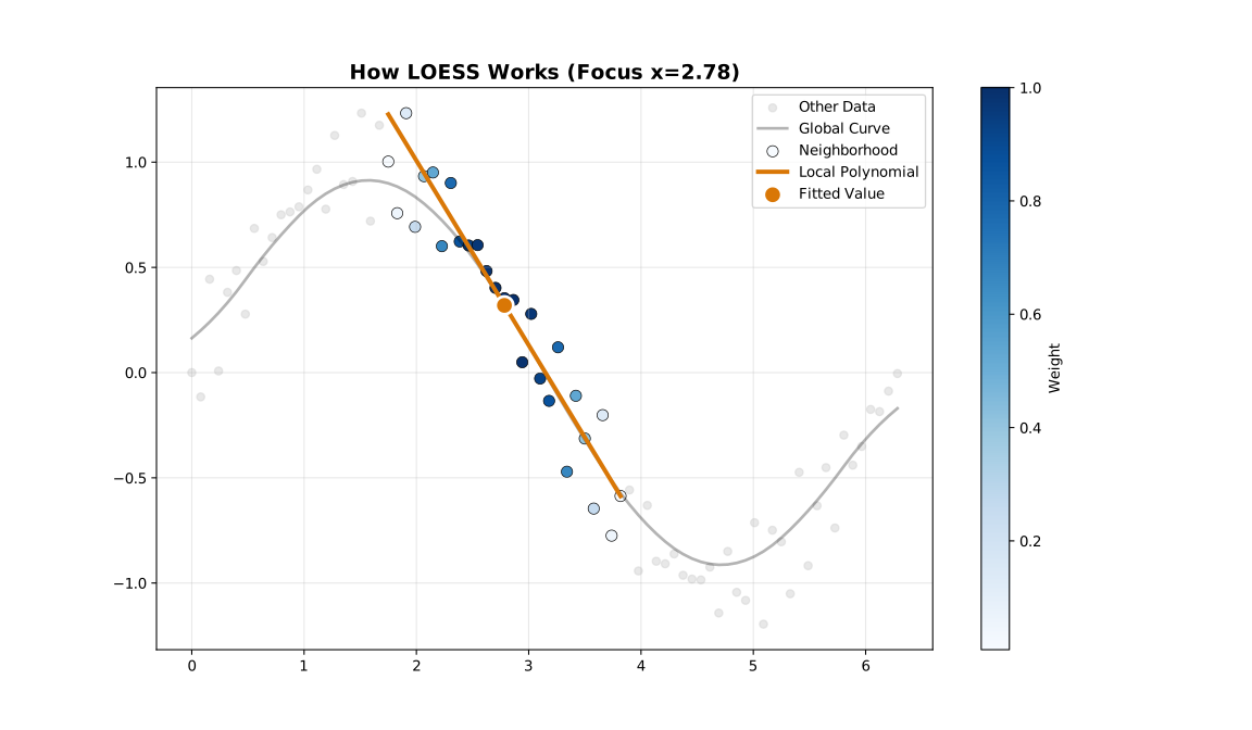
For each point in your data, LOESS:
- Selects neighbors — Choose the nearest points (controlled by
fraction) - Assigns weights — Closer points get higher weights (using a kernel function)
- Fits locally — Perform weighted least squares regression
- Extracts value — Use the fitted value as the smoothed estimate
- Iterates (optional) — Reweight points based on residuals to reduce outlier influence
The Fraction Parameter
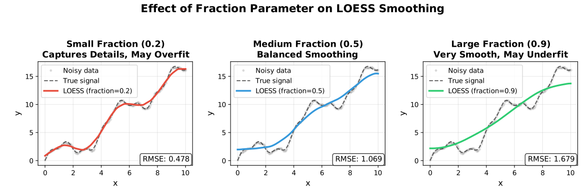
The fraction (also called bandwidth or span) is the most important parameter. It controls what proportion of data is used for each local fit.
| Fraction | Effect | When to Use |
|---|---|---|
| 0.1–0.3 | Fine detail, follows data closely | Rapidly changing signals |
| 0.3–0.5 | Balanced smoothing | Most applications |
| 0.5–0.7 | Heavy smoothing | Noisy data, trend extraction |
| 0.7–1.0 | Very smooth | Strong noise, global trends |
Rule of Thumb
Start with fraction=0.67 (the default) and adjust based on visual inspection. Use cross-validation for automated selection.
Robustness Iterations
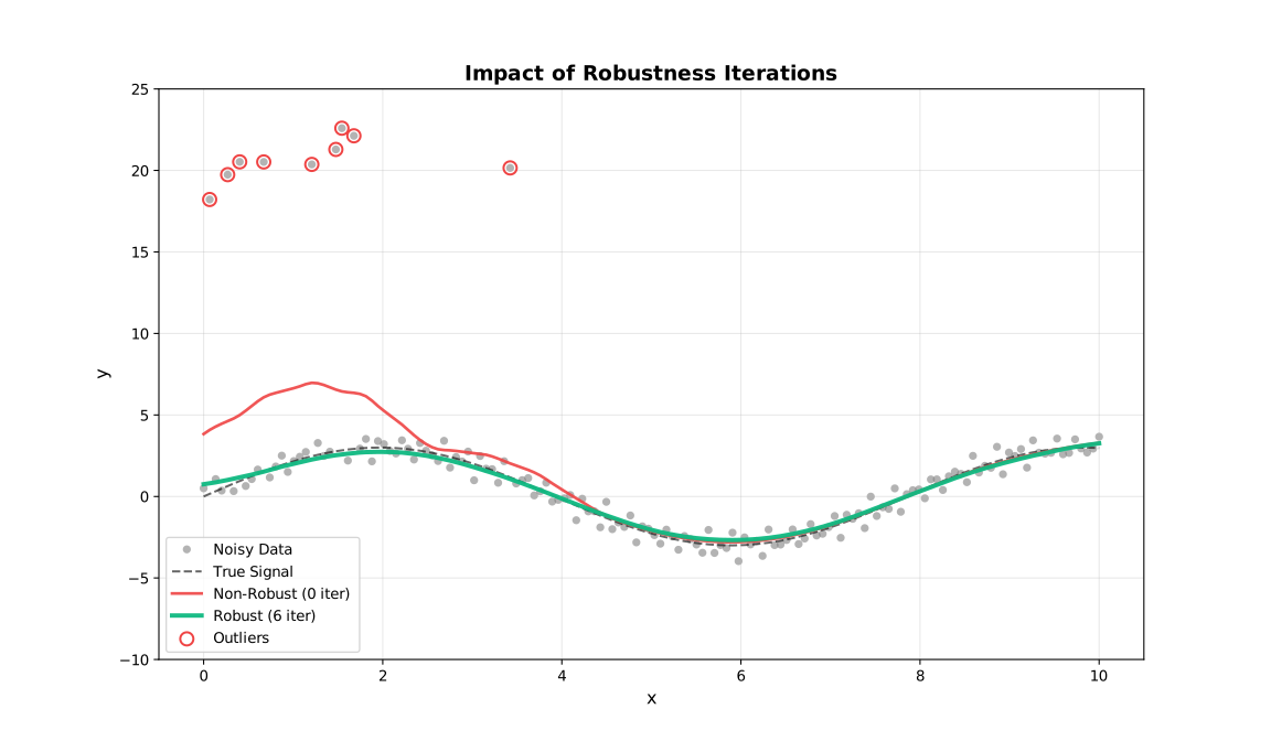
Standard LOESS is sensitive to outliers. Robustness iterations downweight points with large residuals:
| Iterations | Effect | When to Use |
|---|---|---|
| 0 | No robustness (fastest) | Clean data, speed-critical |
| 1–3 | Moderate robustness | Most applications |
| 4–6 | Strong robustness | Data with outliers |
| 7+ | Very strong | Heavy contamination |
Confidence vs Prediction Intervals
| Interval Type | What It Represents | Width |
|---|---|---|
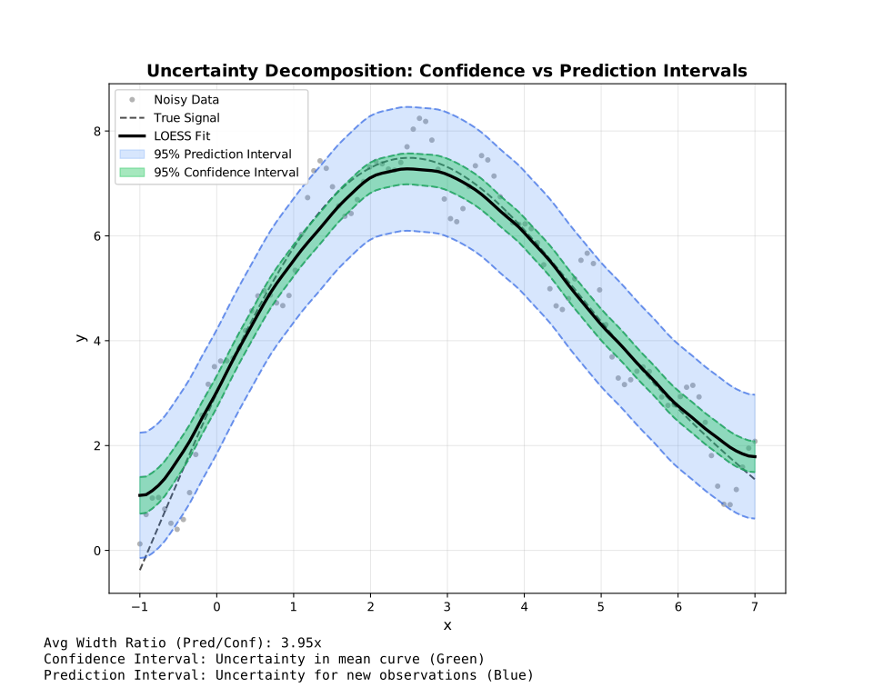
| Confidence | Uncertainty in the mean curve | Narrow |
| Prediction | Uncertainty for new observations | Wide |
- Use confidence intervals to show where the true trend likely lies
- Use prediction intervals to show where new data points might fall
Execution Modes
Choose the right mode based on your use case:
| Mode | Use Case | Memory | Features |
|---|---|---|---|
| Batch | Complete datasets | Entire dataset | All features |
| Streaming | Large files (>100K points) | One chunk | Residuals, robustness |
| Online | Real-time data | Fixed window | Incremental updates |
Key Advantages
| Feature | LOESS | Polynomial Regression | Moving Average |
|---|---|---|---|
| No parametric assumptions | ✓ | ✗ | ✓ |
| Adapts to local structure | ✓ | ✗ | Partial |
| Robust to outliers | ✓ | ✗ | ✗ |
| Uncertainty estimates | ✓ | ✓ | ✗ |
| Handles irregular sampling | ✓ | ✓ | ✗ |
Next Steps
- Quick Start — See it in action
- Parameters — All configuration options
- Polynomial Degree — Constant, linear, quadratic fits
- Multivariate LOESS — 2D and n-D smoothing
- Boundary Handling — Edge bias reduction strategies
- Robustness — Outlier downweighting methods
- Scaling Methods — MAD, MAR, Mean scale estimation
- Merge Strategies — Chunk reconciliation in Streaming mode
- Tutorials — Application-specific guides